Hive and R Playing Nicely Together
Hive is a data warehouse. R is a language for statistics and graphics. Getting these two programs to work together is a beautiful thing.
This post assumes that you already have HDFS, Hive, and Pig running. If there is an interest in seeing a post on how to get these installed and running, please let me know.
Picking a Data Set
Before we can do anything, we need to have a data set. I chose the data from NOAA’s Climate Research Network. Begin by downloading the data from their FTP site. This data set is not too terribly huge - about 600k rows of climate data spread across about 2100 files.
Once downloaded to your local machine, you can upload the data to HDFS with the following command.
$ hdfs dfs -put -f **/*.txt hdfs://localhost:9000/user/climate/raw
Queryable Data with Hive
Having the data in text files in HDFS is a good start, but it is certainly not sufficient for our needs. Apache Avro is a serialization format that can be read by many different tools, including Hive. Another advantage of Avro is that it stores its own schema in the file header, so files are completely portable.
Unfortunately, the *.txt format is a fixed width format. This is not something we can work with out of the box. Fortunately, the Piggybank project has a FixedWidthLoader class that is exactly what we need.
climate = LOAD '/user/climate/raw/**/*.txt' USING org.apache.pig.piggybank.storage.FixedWidthLoader(
  '1-5, 7-14, 16-21, 23-29, 31-37, 39-45, 47-53, 55-61, 63-69, 71-77, 79-86, 88,
   90-96, 98-104, 106-112, 114-120, 122-128, 130-136, 138-144, 146-152, 154-160,
   162-168, 170-176, 178-184, 186-192, 194-200, 202-208, 210-216',
  'USE_HEADER',
  'WBANNO: chararray, LST_DATE: chararray, CRX_VN: chararray, LONGITUDE: float,
   LATITUDE: float, T_DAILY_MAX: float, T_DAILY_MIN: float, T_DAILY_MEAN: float,
   T_DAILY_AVG: float, P_DAILY_CALC: float, SOLARAD_DAILY: float,
   SUR_TEMP_DAILY_TYPE: chararray, SUR_TEMP_DAILY_MAX: float,
   SUR_TEMP_DAILY_MIN: float, SUR_TEMP_DAILY_AVG: float, RH_DAILY_MAX: float,
   RH_DAILY_MIN: float, RH_DAILY_AVG: float, SOIL_MOISTURE_5_DAILY: float,
   SOIL_MOISTURE_10_DAILY: float, SOIL_MOISTURE_20_DAILY: float,
   SOIL_MOISTURE_50_DAILY: float, SOIL_MOISTURE_100_DAILY: float,
   SOIL_TEMP_5_DAILY: float, SOIL_TEMP_10_DAILY: float, SOIL_TEMP_20_DAILY: float,
   SOIL_TEMP_50_DAILY: float, SOIL_TEMP_100_DAILY: float'
  );

rmf /user/climate/avro;
rmf /user/climate/csv;

STORE climate INTO '/user/clmate/avro' USING AvroStorage();
STORE climate INTO '/user/climate/csv' USING PigStorage(',');
This will create our Avro files in HDFS. Hive requires the Avro schema in its own file. Fortunately, there is a Python tool (along with C#, Java, or Ruby) that lets us quickly get the schema.
import avro
import avro.datafile
import avro.io
data_file = 'path/to/avro/part-m-00001.avro'
schema_file = 'path/to/avro/climate.avsc'
file_reader = open(data_file, 'rb')
avro_reader = avro.datafile.DataFileReader(file_reader, avro.io.DatumReader())
schema_writer = open(schema_file, 'w')
schema_writer.write(avro_reader.meta.get('avro.schema'))
schema_writer.close()
Once our data is stored and we have a schema, we can create our Hive table.
CREATE EXTERNAL TABLE climate
ROW FORMAT SERDE 'org.apache.hadoop.hive.serde2.avro.AvroSerDe'
STORED as INPUTFORMAT 'org.apache.hadoop.hive.ql.io.avro.AvroContainerInputFormat'
OUTPUTFORMAT 'org.apache.hadoop.hive.ql.io.avro.AvroContainerOutputFormat'
LOCATION '/user/climate/avro'
TBLPROPERTIES ('avro.schema.url'='hdfs:///user/climate/climate.avsc');
Working with R
The good news is that once your data is stored in Hive, you can use Hive’s JDBC connector to query data as if it were any other database. Begin by loading the necessary libraries.
library(rJava)
library(RJDBC)
Our first task is to update the Java class path. The JDBC driver needs to know where to find classes. This next block of code will do this for us. The directories listed below will be different depending on your platform and installation.
options(java.parameters = '-Xmx8g')
hadoop_jar_dirs <- c('/usr/local/Cellar/hadoop/2.7.3/libexec/share/hadoop/common',
                     '/usr/local/Cellar/hadoop/2.7.3/libexec/share/hadoop/common/lib',
                     '/usr/local/Cellar/hive/2.1.0/libexec/lib')
clpath <- c()
for (d in hadoop_jar_dirs) {
  clpath <- c(clpath, list.files(d, pattern = 'jar', full.names = TRUE))
}
.jinit(classpath = clpath)
.jaddClassPath(clpath)
hive_jdbc_jar <- '/usr/local/Cellar/hive/2.1.0/libexec/lib/hive-jdbc-2.1.0.jar'
hive_driver <- 'org.apache.hive.jdbc.HiveDriver'
hive_url <- 'jdbc:hive2://localhost:10000/climate'
drv <- JDBC(hive_driver, hive_jdbc_jar)
conn <- dbConnect(drv, hive_url)
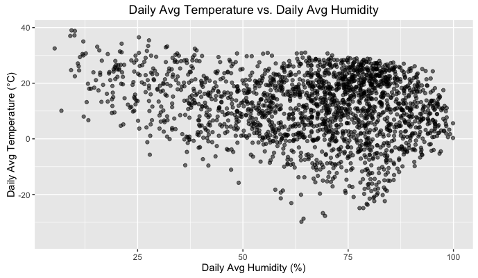
Now that our data is loaded, we produce output as with any other data frame.
sample_size <- 5000
climate.sample <- sample_n(climate, sample_size)
ggplot(data = climate.sample, mapping = aes(rh_daily_avg, t_daily_avg)) +
  geom_point(mapping = aes(alpha = 0.1), na.rm = TRUE) +
  theme(legend.position = 'none') +
  ggtitle('Daily Avg Temperature vs. Daily Avg Humidity') +
  xlab('Daily Avg Humidity (%)') +
  ylab('Daily Avg Temperature (°C)')

Now, you’re all set to analyze your data to your heart’s content!
