Statistics Done Wrong: Understanding Distributions
I recently started reading Statistics Done Wrong: The Woefully Complete Guide by Alex Reinhart. Right from the get-go, the book is a fascinating look at methodology and statistical illiteracy. Thousands of academic papers are published every year by authors who, while they may be experts in their specific fields, have very little statistical training.
In his first chapter, Reinhart demonstrates this problem when discussing p-values. Let’s assume you have a true/false test, and a student has 9 correct answers out of 12. Does the student actually know the material, or did the student just guess? The p-value can guide us in answering this question.
Before continuing, let’s define a p-value. A p-value is the probability of finding the observed result, given that the null hypothesis, \(H_0 \), is true. In context of our question, this should make sense. If we have a 12 question true/false test and have students guess at responses, then we expect the average student to score a 50%, or 6 out of 12. However, because of the nature of randomness, if we collect enough data, we would expect some students to get 0, 1, 2, 3, 4, 5, 7, 8, 9, 10, 11, or 12 questions correct as well.
This ought to be our first interesting conclusion. Statistics tell us a great deal about populations, but they tell us very little about individuals. That said, predictive modeling is a subfield of statistics, where you do try to make conclusive statements about individuals. That, however, is beyond the scope of this post.
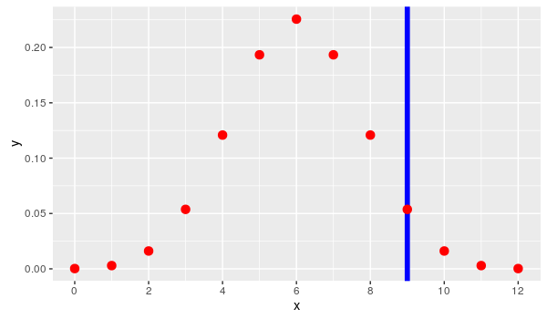
Continuing with the problem at hand, what is the probability that you could randomly guess 12 true/false questions and get 9 correct? We call this the probability density function, or PDF, and we can model this problem with a binomial distribution.
\begin{align}
P(X=k) &= \binom{12}{k}\left(0.5\right)^{k}\left(0.5\right)^{12-k} \
P(X=9) &= \binom{12}{9}\left(0.5\right)^{9}\left(0.5\right)^{3} \
P(X=9) &= 220 \times 0.00195 \times 0.125 \
P(X=9) &= 0.0537
\end{align}
In R, we can get this value much more easily with the dbinom function.
> dbinom(9, 12, 0.5)
## [1] 0.05371094
If we gave this test to 100 students, we would expect about 5 of them to score 9 out of 12.
To compute this p-value, to determine if this score is really different from chance, we need simply compute the upper tail cumulative density of the binomial distribution.
\begin{align} P(X \ge k) &= \sum_{i=k}^{12} \binom{12}{i}\left(0.5\right)^{i}\left(0.5\right)^{12-i} \end{align}
Computing this high tail distribution is done with the pbinom function. It is a little more complicated to express, as it is an infinite series beta function, but the idea is the same. We add up all of the values to the right of the blue line.
> pbinom(8, 12, 0.5, lower.tail = FALSE)
## [1] 0.07299805
This is our p-value. Graphically, this is the cumulative values of the dots to the right of the blue line in the following image.

Reframing the Question
This is not where the author’s story ends. He then asks, what if we presented the data differently? What if the student was allowed to answer questions until he or she got three incorrect responses, and in this scenario, the student got his or her third incorrect response on the 12th question.
Already, we know more information. First of all, we know what the 12th response was incorrect. Second, we know there are more than 12 possible questions. Some students may only be given 3 questions, get all 3 wrong, and their test will be over. It is also possible that some students that some students may be given dozens, hundreds, or even thousands of questions before they get 3 incorrect responses. This time, we ask a slightly different question. What is the probability that a student gets his or third question wrong on the 12th question, given random guessing?
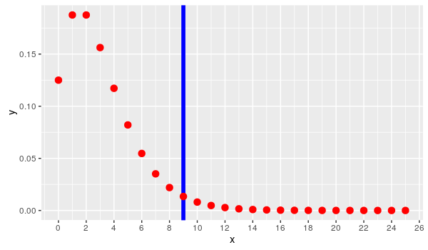
Instead of a binomial distribution, this data set would now follow a negative binomial distribution.
> pnbinom(8, 3, 0.5, lower.tail = FALSE)
## [1] 0.03271484
Note that in our R functions, we use 8 instead of 9 in both of our examples. This is because the binomial and negative binomial distributions are discrete probability functions. They measure to the left, and including the test value. If we want the value plus the values to the right - lower.tail = FALSE - we need to use 8 instead of 9.
Also, the R function is written in a slightly odd way. pbinom(k, r, p) means answering the question, “What is the probability of getting k successes before getting r failures?” Since we are using lower.tail = FALSE we want to know the answer to, “What is the probability of getting 9 or more correct answers before getting 3 failures, when just random guesses are used?”

What makes this result so interesting? We have the exact same data: a student’s score of 9 out of 12. In this scenario, we’re saying that there is only a 3.3% chance that the result could be this extreme.
If we are using \( \alpha = 0.05 \), then our chosen model makes all the difference if we should accept these results as random chance or not. This is why statistical literacy is so vital. How you create your statistical design and how you build your model can make a difference in the result significance and the subsequent interpretation of the study. Not knowing enough about statistics can lead you to proclaim facts that aren’t there or ignore facts that are.
