R Maps: Super Simple Introduction
If you want to work with maps, you’re going to need a shapefile. In short, a shapefile is a list of coordinates that define a polygon. With coordinates, you can define a triangle. Everything else grows more complicated from that basic shape. I used the Zip Code Tabulation Areas from www.census.gov.
I also needed a list of all Indiana zip codes. I have provided one here.
suppressMessages({
    library(broom)
    library(ggplot2)
    library(readr)
    library(rgdal)
})

# Paths to files.
path_to_shapefile <- file.path(".", "tl_2018_us_zcta510", "tl_2018_us_zcta510.shp")
path_to_zip <- file.path(".", "indiana_zip_codes.csv")

# Load list of zip codes. Ensure everything is read as character.
zips <- read_csv(path_to_zip, col_types = c(zip_code = "c",
                                            city = "c",
                                            county = "c"))

# Load the spatial polygons data frame. Keep strings as strings.
spdf <- readOGR(path_to_shapefile, stringsAsFactors = FALSE)
We only want to keep the zip codes in Indiana. To do this, we will filter our spdf data set. The GEOID10 column is the zip code.
# Keep zips, all columns.
filtered_spdf <- spdf[spdf$GEOID10 %in% zips$zip_code,]
Next, run broom::tidy() to turn our shapefile into a proper data frame that can be consumed by ggplot. I tried running this on the entire (unfiltered) shapefile, and it crashed out R Studio.
tidy_df <- tidy(broom_df, region = "GEOID10")
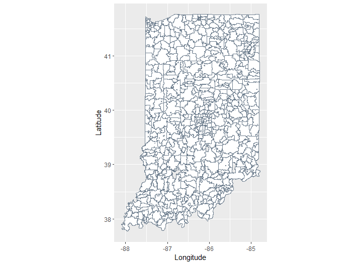
Finally, the only task remaining is to create our plot.
ggplot(data = tidy_df, aes(x = long, y = lat, group = group)) +
    geom_polygon(color = "slategray", fill = "white") +
    coord_quickmap() +
    xlab("Longitude") +
    ylab("Latitude")
Here’s the final result.

I hope this helps you get started with mapping in R.
